Building geometry solvers for the IMO Grand Challenge
(Dated: Sep 15 2020)
Synthetic geometry lies at the intersection of human intuition—insights arising from our core knowledge priors of shape, symmetry, distance, and motion—and formal proof: for two millenia, the treatment of geometry in Euclid’s Elements has exemplified the axiomatic method in mathematics.
While not actively researched in contemporary mathematics, synthetic geometry survives today in the form of olympiad geometry problems posed in contests like the International Mathematical Olympiad (IMO). While in principle reducible to the axiomatics of Euclid, olympiad geometry in practice is situated on its own foundations and a body of assumed knowledge which goes far beyond the axioms in the Elements: reduction to real/complex/barycentric coordinates, algebraic methods a la Gröbner bases, and passage to projective or inversive geometry, to name a few tricks. Modulo this assumed knowledge, proofs in olympiad geometry remain elementary and relatively short. However, they often require creative insights on when to apply techniques that can transform the search space—a single well-chosen auxiliary point or a clever inversion can cut a path through an otherwise intractably thorny problem.
As such, synthetic geometry poses an enticing challenge for artificially intelligent theorem proving. On one hand, the insight required for well-chosen auxiliary points and transformations, and the ability to finish a proof given such insights, are miniaturizations of the problems of goal-conditioned term synthesis (given a theorem to prove, what intermediate definitions or lemmas will lead to a proof?)—and tactic selection. On the other hand, geometry is remarkably accessible: anyone can draw a diagram to gain intuition about a problem, or perturb diagrams to quickly discover new problems. Put another way, geometry distinguishes itself by the ease with which humans can synthesize and manipulate models to guide reasoning, motivate constructions, and discover interesting facts. Moreover, we can be fairly confident in a conjecture \(\phi \to \psi\) if we have sampled merely a few dozen diagrams satisfying \(\phi\) as pathologically as possible and find that in all of them, \(\psi\) also holds. Since it turns out to be easy to automatically synthesize high-quality diagrams (paper), this means that in geometry, it might be feasible to trade compute for a curriculum—definitely not something we can say for e.g. arithmetic geometry (it took a team of mathematicians months to formally construct a single perfectoid space in Lean) or elementary number theory, whose logic is somehow less tame than geometry’s, and where it is really easy to conjecture really hard problems (and where counterexamples to conjectures can show up after billions of positive examples.)
I spent the summer working on geometry solvers for the IMO Grand Challenge with Dan Selsam at Microsoft Research. A superhuman olympiad geometry solver will only be 1/4th of a solution to the IMO Grand Challenge, but we expect the techniques developed here to accelerate the development of solvers for the other problem domains. What follows is a (not-so-brief) field report of what we’ve tried and learned so far.
The agony and the ecstasy of forwards vs backwards reasoning
One of the fundamental dichotomies of automated reasoning—and a source of many tough design decisions—is between forwards and backwards reasoning. Should one derive consequences of facts already known, or work backwards from the goal to narrow the search space before proceeding? Put another way, should one build the proof tree from the leaves up (forwards) or from the root down (backwards)? Either approach has drawbacks: forwards reasoning can produce many unpromising intermediate lemmas, leading to problems of memory complexity; conversely, backwards reasoning can explore many unpromising branches of the search tree, leading to problems of time complexity.
The best results seem to arise from combining both. Humans, for example, rarely use pure forwards or backwards reasoning alone. In practice, we rely on instinctual heuristics for when to forward-chain into promising parts of the search space and when to expand the backwards search tree (i.e., accumulating a table of lemmas that we know can finish the proof as soon as we supply their preconditions). Sometimes our intuition tells us it’s a good idea to just unwind definitions and follow our nose, and other times we’ll somehow know we’re in a bad part of the search space and should reorient with another technique.
SAT solving is a great example. One can think of the DPLL algorithm for SAT as performing a backwards search for a resolution proof tree rooted at the empty clause. (If the first variable selected is \(x\), then this is a promise that the final resolution yielding the empty clause \(\varepsilon\) is that of the unit clauses \((x)\) and \((\neg x)\).) Unlike first-order logic, this resolution proof search is guaranteed to terminate, but the runtime can easily blow up if we do not prune (for example, suppose we disable unit propagation). Now consider the extension of DPLL to CDCL. A learned clause \(C\) produced by conflict analysis of a candidate assignment \(\mathcal{F}|_{\alpha}\) can be proved from \(\mathcal{F}\). In terms of the resolution proof, every time we close a branch of the backwards search from \(\varepsilon\), we also perform a bit of forwards reasoning, accumulating a proof forest starting at the leaves which lets us close future branches of the backwards search more quickly. In practice, CDCL vastly reduces the time complexity of DPLL. This comes at the cost of intricate heuristics (clause activity scores, glue levels…) for managing the memory complexity of the accumulated lemmas. Nevertheless, this is a paradigmatic example of how forwards and backwards reasoning can be synthesized to great effect.
Tabled resolution in logic programming is another example. Backward chaining with Horn clauses (e.g. Prolog) is the prototypical backwards reasoning algorithm. Naïvely implemented, it also illustrates the pitfalls of pure backwards reasoning. Without storing information of what we have already proved in a global state which persists across different branches of the search (in this case a table for memoization; in the case of CDCL, a clause database), the search thrashes and blows up; in the case of Prolog (or systems that use vanilla SLD resolution, like Lean 3’s typeclass system) it can even loop. Tabling maintains a search forest instead of a single backtracking search tree. This can be viewed as incorporating forwards reasoning (goal propagation and scheduling) into a purely backwards algorithm: failed search trees from earlier in the search are suspended instead of discarded, and can be resumed if their dependencies are discovered and propagated from another part of the search later on.
SearchT: a monad transformer for generic backwards search
One of the tools we developed this summer is a monad transformer for generic backwards search, called SearchT.
data SearchT cp c m a = SearchT (m (Status cp c m a))

data Status cp c m a =
    Fail
  | Done a
  | ChoicePoint (Decision cp c m a)

data Decision cp c m a = Decision { choicePoint :: cp,
                                    choices     :: [(c, SearchT cp c m a)] }
A value of type SearchT cp c m a represents a monadic computation in m that searches for a value of a. When this monadic computation is executed, a SearchT program either fails, succeeds with a desired value of type a, or returns a choice point, which wraps a list of continuations representing possible branches of the search with features of type cp and c to be consumed by heuristics. The value returned by the search is completely general; a could even be a SearchT program itself, so that the whole thing is metasearch over search programs. Unlike ListT, which can also be thought of as encoding a search, the continuations in SearchT are explicit and the search must be run explicitly. The benefit of running the search ourselves is that now it doesn’t have to be depth first (as in ListT) and we can manage the continuations in whatever container (stack, queue, priority queue…) we like. In between processing branches of the search, we can also process the arbitrary features returned by the choice points as input to branching heuristics. For example, at a high level, the breadth-first search in the outer loop of DeepHOL, where possible choices of tactic applications are re-ordered according to a policy network, can be encoded this way.
Global state which persists across different branches of the search can be maintained in the inner monad m. For example, m could be a StateT ProofForest IO, and a SearchT program could search for terms which unify with the left hand side of a forward chaining rule, apply the rule, and store the result in the global state. In this way, we can implement forward reasoning. Conversely, local state (like a partial proof tree, say, or a cache of local assumptions) that is destroyed upon backtracking can be maintained in an outer state monad, e.g. StateT TacticState (SearchT m cp c a).
We had several uses for the SearchT abstraction—notably, in our ARC solver (which I will describe next), and for mining constructions and conjectures from geometry diagrams.
Warm-up: The Abstraction and Reasoning Challenge (ARC)
The first thing I worked on was a solver for Kaggle’s Abstraction and Reasoning Challenge. The task was to build a solver that could pass what was essentially a battery of psychometric intelligence tests (see Francois Chollet’s preprint for more motivation). Here’s a typical task:
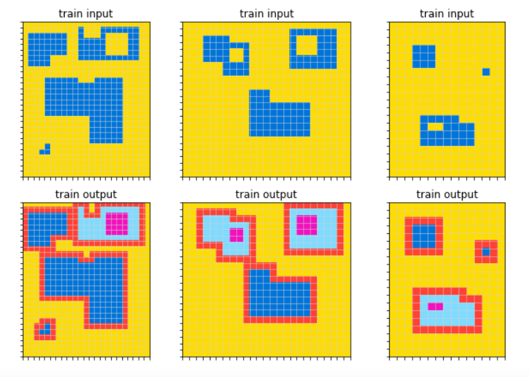
This is an unforgiving few-shot learning problem: there are only a handful of training examples per task, and the answers for the test inputs, including the exact grid dimensions, have to be an exact match.
Our solver was structured around SearchT and performed primarily backwards search, with lightweight caching in a global state. We essentially stored the problem statement and some local assumptions in a search-thread-local state, but ended up passing that around explicitly. The core definitions are quite simple (for simplicity, we suppress the choice point datatypes in SearchT):
data Goal a b = Goal {
  inputs     :: Ex a, -- bundles train inputs and test inputs
  outputs    :: [b], -- train labels
  synthCtx   :: SynthContext -- local context
  }

type StdGoal   = Goal (Grid Color) (Grid Color)

data SolverContext = SolverContext { ctxChecksum :: String }

data SolverState = SolverState {
  visitedGoals   :: Set StdGoal,
  parseCache     :: Map (Grid Color, Parse.Options) [Shape Color] }

type CoreM  = ReaderT SolverContext (StateT SolverState IO)
type SolveM = SearchT CoreM
Thus, given a StdGoal, we wish to search for output grids for the test inputs, i.e. execute a SolveM [Grid Color]. As SearchT is generic, one can execute a nested search for arbitrary data from inside of a SearchT program. This arose occasionally in ARC, for example when we wanted to synthesize a function from Int features for each input grid to some Int for each of the output grids. We handled this sort of task through a synthesis framework built around SearchT, motivated by deductive backpropagation. Here’s a prototypical example. Most of our Int -> Int synthesis tasks were handled by a function called synthInts2IntE, which is called with a list of Int features extracted from the problem, and uses SearchT to perform a top-down search for an arithmetic expression \(E\) which explains a list of training examples and produces test outputs. Every time this search branches, i.e. guesses what the next operation of \(E\) is, it propagates this guess to the training examples before recursing. For example, if for all training examples (x,y) the guess is that y = x + ?k, then before recursing we transform the training examples to (y - x, ?k), and check if ?k is exactly one of the precomputed Int features, or constant across all training examples. In this way we can explain arbitrarily complicated arithmetic expressions of Int features, like if the number of columns of the output grid is always \(3 N + 2\) where \(N\) is the number of red pixels in the input grid. We used synthInts2IntE to guess pixel positions, output grid dimensions, and tiling data. Here’s an example of it in action, from our test suite.
testSynthInts2IntE = describe "testSynthInts2IntE" $ do
  let phi1   = ("ascending",  0, Ex [1, 2, 3] [4, 5])
  let phi2   = ("descending", 0, Ex [3, 2, 1] [5, 4])
  let phi3   = ("random",     0, Ex [1, 7, 3] [2, 6])
  let phi4   = ("multiples",  0, Ex [10, 30, 20] [70, 60])
  let phi5   = ("mod3s",      0, Ex [4, 7, 11] [0, 1])
  let inputs = [phi1, phi2, phi3, phi4, phi5]

  it "const/input" $ do
    find1 synthInts2IntE (ESpecType inputs [40, 60, 120]) `shouldBe` [[24, 30]]
Above, input is the list of Int features discussed previously. synthInts2IntE successfully infers that the function is \(x \mapsto 120/x\) and that it should be applied to the input feature phi2.
ARC was really fun, if a bit of a trial by fire. I joined the team—consisting of Dan and Ryan Krueger, a new grad from UMich—three weeks before the submission deadline, had just spent months welding graph neural networks onto SAT solvers written in C++, and hadn’t touched Haskell in a year. The Haskell solver didn’t even exist until a few days before I joined, when Dan started a port from an earlier prototype in Lean 4. There were many things we could have done better, like making our search procedures more compositional and avoiding overfitting to the training data, but considering all the crazy stuff we were trying—like a generic program synthesis framework written in SearchT, or that afternoon I wasted trying to use discrete Fourier transforms for tile imputation—we did quite well, placing in the top 2% out of more than 900 submissions.
Designing geometry solvers
Our first attempt at a geometry solver was also based on SearchT with purely backwards reasoning. We quickly found out that without good heuristics for expanding the search tree, we hit blowups whenever we had to do transitivity reasoning. Suppose that the goal is p = q, and we want to expand this node of the search tree by applying the transitivity rule of equality x = y → y = z → x = z. This naïvely adds as many branches as there are points in the problem, so without good heuristics for instantiation, the solver can get lost for a long time in hopeless parts of the search space before it realizes it has to backtrack. The problem is even worse for backwards reasoning with collinearity or concyclicity predicates. The analogous rule for concyclicity, for example, is cycl p q r s → cycl q r s t → cycl p q r t ∧ cycl p q s t ∧ cycl p r s t. So, if the goal is to prove cycl a b c d, then backwards chaining naïvely adds \(\binom{n}{3}\) new branches (where \(n\) is the number of points). What if a proof requires multiple concyclicity assertions (as is often the case)? Obviously, we needed to try something better.
We came up with two answers for this problem:
-
Trade memory for time by integrating a forward chaining module that could efficiently represent and propagate equality, collinearity, and concylicity facts. Don’t let backwards search threads branch on transitivity lemmas; instead, suspend them and resume when the forward chainer has learned the required facts.
-
Use better, model-driven heuristics to instantiate lemmas, avoiding easily-prunable parts of the search space. A human would never try to prove that some points are concylic if they are obviously not concyclic in a diagram—so, if our solver is able to synthesize diagrams, why don’t we do the same?
\(k\)-equivalence relations and associated algorithms
While there are well-tested techniques for forward chaining with equality, i.e. storing (i.e. union-find datastructures), propagating (i.e. congruence closure), and producing proofs (i.e. proof forests) about a sequence of equality assertions, these do not transpose efficiently to the case of lines and circles. For instance, if we know the collinearities coll a b c, coll b c d, and coll c d e, we can conclude \(\binom{5}{3}\) collinearity facts. If we introduce a new function symbol ℓ : Point -> Point -> Line, the situation doesn’t really change, as we now have to process \(\binom{5}{2}\) (choose 2) line equalities instead. We tried some experiments saturating collinearity/concyclicity facts this way in Z3 and it ground (pun maybe intended) to a halt.
Of course, no human thinks of coll a b c ∧ coll b c d as a sequence of line equalities ℓ a b = ℓ a c = ℓ a d = ℓ a e = .... Instead, we recognize the collection of all those points as forming a line entity, such that two line entities are merged whenever they share two points. It turns out this intuition has an interesting theoretical basis. Our quest for efficient line and circle management led us to the abstract concept of a \(k\)-equivalence relation, which captures collinearity and concyclicity as the special cases of \(k = 2\) and \(k = 3\). Fix a set \(X\). We say that a predicate \(R\) on \(X^{k+1}\) is a \(k\)-equivalence relation on \(X\) if it satisfies the following properties:
- (sub-reflexivity) For every \(\vec{x} = (x_1, \dots, x_{k+1}) \in X^{k+1}\), if some \(x_i = x_j\), then \(R(\vec{x})\).
- (permutation-invariance) For every \(\sigma \in \mathrm{Sym}(k+1), R(\vec{x}) \iff R(\sigma(\vec{x}))\).
- (\(k\)-transitivity) For all \(x_1, \dots, x_k\), \(y_1, y_2\), if \(R(\vec{x}, y_1)\) and \(R(\vec{x}, y_2)\), then for any \(i\), \(R(x_1, \dots, x_{i-1}, x_{i+1}, \dots, x_{k}, y_1, y_2)\).
Interestingly, every \(k\)-equivalence relation \(R\) on \(X\) induces an actual equivalence relation \(E_{R}\) on \(X^k\). The proof is reminiscent of arguments involving the Steinitz exchange property in matroids. The classes of these equivalence relations are furthermore represented by subsets of \(X\), which we call \(k\)-sets. The \(k\)-sets are precisely the line and circle entities that we want to use for managing collinearity and concyclicity facts.
To distinguish them from the EClass datastructures used by the congruence closure module, we use the term KClass. A KClass is owned by the forward chaining module, and comprises a set of terms and some metadata. Integrating KClass reasoning with EClass reasoning is nontrivial because equality assertions propagated by the congruence closure module can trigger KClass merges. Extra care is required because a KClass with \(n\) terms is an abbreviation for an EClass with \(\binom{n}{k}\) terms to which the congruence closure module does not really have access. In the presence of point-valued function symbols on lines and circles (for example, the operation of taking the center of a circle), these KClass merges can propagate new equality assertions, and so on.
In forthcoming work, Dan and I actually work out a general proof-producing decision procedure for arbitrarily nested \(k\)-equivalence relations (i.e., where we treat \(k\)-equivalence relations on \(k\)-sets themselves, e.g. circular bundles of lines), a special case of which is used in our solver. Producing proofs is not as easy as it is in the \(k=1\) case of equality, because while an EClass only has to chain together some of the equality assertions it sees in order to justify why two points are equal, a merge of \(K\)-classes abbreviates many \(k\)-transitivity assertions involving points from both classes which are never made explicit, and which must be reconstructed.
Multi-sorted language with function symbols
It is possible to formulate synthetic geometry using only points, without the addtional sorts required for quantification over lines and circles. It’s also possible to eliminate function symbols, replacing them with their graph relations. In early versions of the solver, we worked in a single-sorted point-only language with no function symbols because it seemed to simplify the implementation. In retrospect, this was a mistake on two fronts.
The first is diagram-building. Using only points seems like a great idea at first glance—it minimizes the API surface area, and the only information which has to be transmitted between the diagram-builder module to the solver is a list of low-level constraints (when requesting a diagram) and a list of (point name, coordinates) pairs (when serving a diagram). But, it turns out that SymPy (and later, TensorFlow) has a harder time solving for e.g. “the set of points which satisfy the property of being on the radical axis of two circles”, especially when stacked with a dozen other constraints in multiple variables, than simply computing the exact equation of the radical axis, which we know how to do. At one point we ended up with an extremely clever compiler which would accept a point-only formulation of a problem, analyze it to detect the function symbols we were skolemizing, and compile them to an IR so that the diagram builder would know what could be computed or parametrized and what had to actually be solved—code that evaporated when we enabled support for function symbols, as the diagram builder could then just recurse on the term it was finding coordinates for.
The second, related to the first, is handling auxiliary constructions in the solver. In a point-only language, we are forced to replace function symbols (e.g., the perpendicular bisector of segment \(AB\)) with skolemizations instead (“there exists a point \(P\) and a point \(M\), such that \(M\) is equidistant from \(A\) and \(B\) and \(PM\) is perpendicular to \(AB\)…”). On one hand, this has the benefit of forcing us to be very explicit when introducing new constructions, as they have to be introduced in terms of fresh variable and new constraints. On the other, using skolemizations obscures the composition of constructions (e.g. “the intersection of the perpendicular bisector with the internal angle bisector of \(\angle P Q R\)”) and muddles the action space for learning a policy to add new constructions—a function symbol can be thought of as a high-level abbreviation for a skolemized point and its associated properties.
Finally, working in a point-only language makes solving some problems extremely awkward. Consider the following problem:
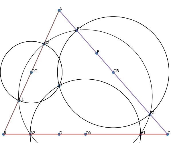
(IMO 2008 P1) Let \(H\) be the orthocenter of an acute-angled triangle \(ABC\). The circle \(\Gamma_A\) centered at the midpoint of \(BC\) and passing through \(H\) intersects line \(BC\) at points \(A_1\) and \(A_2\). Similarly, define the points \(B_1, B_2, C_1\) and \(C_2\). Prove that six points \(A_1, A_2, B_1, B_2, C_1\) and \(C_2\) are concyclic.
One solution is to apply the power of a point theorem to conclude that any two out of the three pairs \((A_1, A_2), (B_1, B_2), (C_1, C_2)\) are concyclic, then to show that those three circles are actually equal by taking perpendicular bisectors. In a point-only language, this leads to contrived skolemizations for points on the perpendicular bisectors (as mentioned above) just so we can talk about a line we know how to define; furthermore, what should be a straightforward chain of equality assertions (after realizing taking perpendicular bisectors is the right thing to do) is indirected through a mess of concyclicity assertions, because we can’t say that two circles are equal, only that there exist four points, three of which are shared by both circles.
Using models
Diagrams are an essential component of human reasoning for synthetic geometry problems. Importantly, we use them to make conjectures, perform premise selection, and update our value estimates. For example, in the following problem:
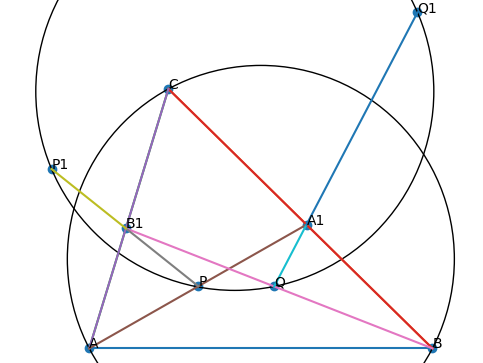
(IMO 2019 P2) In triangle \(\Delta ABC\), point \(A_1\) lies on side \(BC\) and point \(B_1\) lies on side \(AC\). Let \(P\) and \(Q\) be points on segments \(A A_1\) and \(B B_1\) respectively, such that \(\overline{PQ}\) is parallel to \(\overline{AB}\). Let \(P_1\) be a point on line \(P B_1\) such that \(B_1\) lies strictly between \(P\) and \(P_1\), and \(\angle P P_1 C = \angle B A C\). Similarly, let \(Q_1\) be a point on line \(Q A_1\) such that \(A_1\) lies strictly between \(Q\) and \(Q_1\) and \(\angle C Q_1 Q = \angle C B A\). Prove that points \(P\),\(Q\), \(P_1\) and \(Q_1\) are concyclic.
our eyes are drawn to the second points of intersection \(A_2\) of \(\overline{A A_1}\) (resp. \(B_2\), \(\overline{B B_1}\)) with the circumcircle of \(\Delta ABC\), because they look like they also lie on the circle we are interested in. After using the diagram to notice these points, we can intuit that at a purely symbolic level, \(A_2\) and \(B_2\) are good points to introduce because they somehow bridge the angles owned by the circumcircle of \(\Delta ABC\) with those owned by the circle through \(P_1 P Q Q_1\), and we will probably need to angle-chase with the inscribed angle theorem to conclude concyclicity. Indeed, as soon as \(A_2\) and \(B_2\) are introduced, the problem reduces to an angle-chase.
Diagram synthesis with TensorFlow
It turns out it’s actually easy to synthesize diagrams for synthetic geometry problems. Our first diagram-builder tried to compile problem statements into multivariate polynomial constraints amenable to exact solution by SymPy and SciPy, but it was brittle, no matter how cleverly we tried to massage the compilation process. Over a weekend in July, Dan and I reworked the diagram-builder module from the ground up, from a completely different direction: we would compile problem statements into computation graphs in TensorFlow instead, using computational geometry know-how to pick good initial values and fix as many degrees of freedom as we could. Then, we would use stochastic gradient descent to go the last mile where symbolic solving couldn’t.
It worked brilliantly—essentially out of the box (in fact, it’s responsible for every diagram in this blog post). It can turn a formally specified problem statement like this:
(declare-points P0 P1 P2 P3 P4 Q0 Q1 Q2 Q3 Q4 M0 M1 M2 M3 M4)
(assert (polygon P0 P1 P2 P3 P4))
(assert (interLL Q1 P0 P1 P2 P3))
(assert (interLL Q2 P1 P2 P3 P4))
(assert (interLL Q3 P2 P3 P4 P0))
(assert (interLL Q4 P3 P4 P0 P1))
(assert (interLL Q0 P4 P0 P1 P2))
(assert (cycl M1 Q0 P0 P1))
(assert (cycl M1 Q1 P1 P2))
(assert (cycl M2 Q1 P1 P2))
(assert (cycl M2 Q2 P2 P3))
(assert (cycl M3 Q2 P2 P3))
(assert (cycl M3 Q3 P3 P4))
(assert (cycl M4 Q3 P3 P4))
(assert (cycl M4 Q4 P4 P0))
(assert (cycl M0 Q4 P4 P0))
(assert (cycl M0 Q0 P0 P1))
(prove (cycl M0 M1 M2 M3 M4))
into a diagram like this in a couple of seconds:
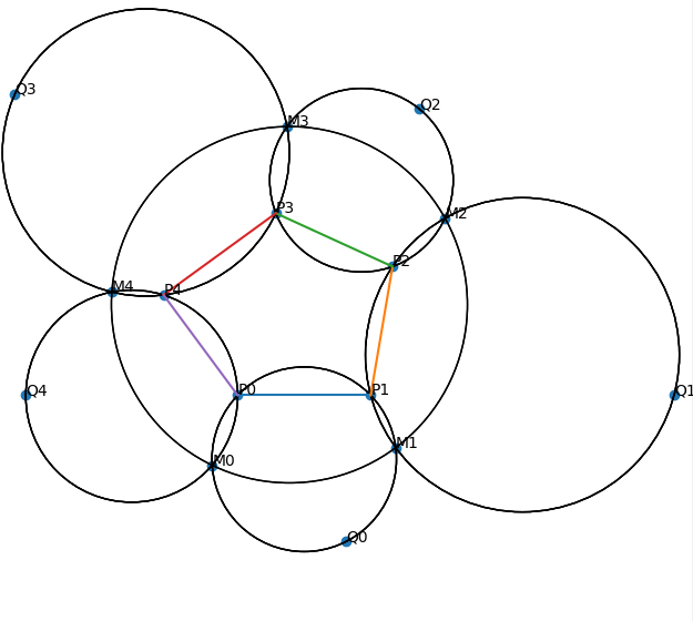
The beautiful thing about this is that different parts of the computation graph can be composed together to represent arbitrarily complicated constructions. If we want, say, the inversion of the arc-midpoint of \(A\) opposite \(B\) about the circumcircle of \(\Delta XYZ\) to be on the perpendicular bisector of \(PQ\), we only need to add another collinearity loss involving the relevant TensorFlow ops to the loss term. I should mention that this is a perfect use-case for static computation graphs—we really want to compile the problem to TensorFlow ops first, so that we can cache ops and re-use them when, for example, the same term is subject to multiple constraints.
Model-based conjecturing
Now, suppose that we have a high quality diagram of a geometry problem; what do we do with it? One thing we can do is run our solver to saturation or a fixed timeout on the problem, look at the resulting forward chaining database, and compare it to what we can read off of the diagram. Any interesting conjectures must be among those properties which are true in the diagram (which, by the soundness theorem, satisfies every property provable from the assumptions) but not yet in the forward chaining database (meaning that it taxes the ability of our solver).
Unsurprisingly, this too can be phrased in terms of a SearchT program. This time, the search is over the problem specification language itself—either for propositions (conjectures) or terms (constructions). We re-use the same error functions from the TensorFlow-based diagram builder and accept propositions if their error is lower than a fixed threshold. At the same time, we maintain a copy of the latest forward-chaining database in a global state, using it to filter out candidate conjectures which were already proved.
Similarly, we can use heuristics to pick out promising constructions. It is important to select good constructions, because adding many new terms can drastically slow down the progress of the forward chainer, because it will then have many new instantiations to consider for each of the forward chaining rules. Specifically, we prefer terms which are involved in the nontrivial conjectures—if the diagram shows that two circles are equal while the forward chainer has not yet merged them, for example, then it is a good bet that constructed points that lie on both circles in the diagram will be involved in the concyclicity assertion that will eventually merge them.
This suggests the following outer loop for automated conjecturing/curriculum generation:
- sample an initial configuration (and as many models as necessary to achieve a desired confidence of completeness)
- forward chain with the solver to a fixed timeout
- enumerate (or learn a policy for sampling) properties which hold in all the diagrams
- filter out the proved conjectures and add the remaining ones as conjectures for training.
This procedure is not particular to synthetic geometry; it applies wherever it is cheap to synthesize models. However, the sample complexity to obtain good conjectures might be much higher than in geometry. For example, there is an analogous model-based conjecturing task for propositional CNF formulas. By the completeness theorem for propositional logic, \(\vdash \phi \to \psi\) if and only if for all assignments \(M\) of all free variables in \(\phi\) and \(\psi\), \(M \vDash \phi \to M \vDash \psi\). Therefore, if we are only given \(\phi\), we can sample a collection \(M_i\) of satisfying assignments of \(\phi\) (which might be easier than proving \(\phi \land \psi\) unsatisfiable) and then read off a sequence of clauses \(C_i\), each of which is satisfied by all the models \(M_i\). Then \(\vdash \phi \to \bigwedge C_i\) is the new conjecture. Satisfying assignments for propositional CNFs are far more likely to give rise to spurious conjectures than geometric diagrams. There might be special problem distributions where it’s easier to sample sufficiently “dense” collections of satisfying assignments.
Model-guided reasoning
In addition to suggesting new conjectures or constructions to consider, models give a convenient way to quickly prune branches of the search (at the cost of some quick numerical lookahead). This is especially important in backwards reasoning; the conclusion of a rule can unify with the solver’s current goal, but the preconditions might be completely unsatisfiable, meaning that any further work along that branch of the search will be wasted.
This inspired a technique that we call diff-chaining, which combines the selection of constructions involved in empirically-observed-yet-symbolically-unproven propositions (the diff) with quickly pruning branches of search that will fail anyways. This works by incorporating backwards reasoning into each step of the forward chaining loop. Given a forward chaining rule of the form \(P_1 \to \dots \to P_k \to Q\) with preconditions \(P_i\) and conclusion \(Q\), we isolate the “existential” variables in the preconditions which do not occur in the conclusion. We then search for instantiations of the conclusion \(Q\), propagating these instantiations to the preconditions; as soon as a precondition becomes ground, its empirical error is checked, and if any precondition is empirically false, we move on to the next rule. If all ground preconditions pass the diagram check, we proceed to instantiate the “existential” variables only with terms involved in the diff.
Conclusion
Reid Barton once told us that one of his tricks for dealing with contest math problems was to assume the conclusion and reason forwards from it, producing easier auxiliary problems whose solutions might hint at the real thing.
In a sense, the IMO Grand Challenge is an instance of this heuristic at extreme scale: after all, push-button automation capable of (1) winning a Millenium Prize certainly implies push-button automation capable of (2) winning gold at the IMO. Naïvely working backwards from a goal might lead to an intractable search space, but the right goal at the right time can motivate the right work: after spending a summer working on one solver motivated by the IMO Grand Challenge after another, I might not know what (1) will look like, but I’ve got a good sense of what (2) will look like, and I think we have a good shot at getting there.